Scalable Bayesian inference in Python
On how variational inference makes probabilistic programming ‘sustainable’
View this on Medium too
Last year I came across the Edward project for probabilistic programming, which was later moved into Tensorflow (in a dev branch). Among the publications listed on the website, one caught my attention as it reported a truly innovative way (to my knowledge at least) to perform variational inference. Its title speaks for itself: “Black box variational inference”, Rajesh Ranganath, Sean Gerrish, David M. Blei.
When performing Bayesian inference we wish to approximate the posterior distribution of the latent variables given some data/observations x (): problem is, the integral is often intractable and numerical methods must be used (just so you know, a latent variable is everything ranging from a discrete variable for a Gaussian mixture model to beta coefficients in a linear regression model or the scale parameter of the posterior distribution of a non-conjugate bayesian model)…
Characterization of the posterior is usually performed using Markov Chain Monte Carlo methods (yes, they come in different flavors), by repeatedly sampling from the (possibly super-complex and multivariate) posterior to build a reliable expectation of the distribution.
With variational inference instead, the basic idea is to pick an approximation
to the posterior distribution from some tractable family, and then try to make this approximation as close as possible to the true posterior,
: this reduces inference to an optimization problem.
The key idea is to introduce a family of distributions over the latent variables z that depend on variational parameters λ, , and find the values of λ that minimize the KL divergence between
and
.
The most common model used in this context is the mean field approximation, where q factors into conditionally independent distributions each governed by a set of parameters (represented here by λ):
.
Minimizing the KL divergence between q(z/λ) and p(z/x) i.e. roughly said, making these distributions as ‘close’/similar as possible is equivalent to maximizing the Evidence Lower Bound (ELBO), calculated as:
calculated w.r.t q(z).
We just need to maximize this expression to find the parameters λ that make the KL divergence small and our q(z/λ) very similar to p(z/x). So where is the catch? Deriving gradients for complex functions is a tedious process, and for sure it is one that cannot be easily automated.
We can solve this problem by using the “black box” variational model reported in the publication cited above: “From the practitioner’s perspective, this method requires only that he or she write functions to evaluate the model log-likelihood. The remaining calculations (properties of the variational distribution and evaluating the Monte Carlo estimate) are easily put into a library to share across models, which means our method can be quickly applied to new modeling settings.”
Let us see how this works: the key idea from the publication is that we can write the gradient of the ELBO as an expectation:
And here come the good part: we can use Monte Carlo to obtain a noisy estimate of this gradient expression: we initialize the model parameters λ (randomly), we sample from q(z/λ), we evaluate the entire expression (see below) and take the mean over different samples. We then use stochastic gradient descent to optimize (maximize) the ELBO!
Black box variational inference for logistic regression
Let us now build a simple model to solve Bayesian logistic regression using black box variational inference. In this context,the probability is distributed as a Bernoulli random variable, whose parameter p is determined by the latent variable z and the input data x (
) which goes through a sigmoid ‘link’ function.
According to the mean field approximation, the distribution of q over z (
) is equal to the product of conditionally independent normal distributions (
), each governed by parameters mu and sigma (
)
Let us try to decompose the gradient of L(λ) to show how we can evaluate it for logistic regression:
: we need to derive the gradient of q w.r.t to mu and sigma. I only report here the gradient of mu (the gradient of sigma follows the same concept and can be found here):
With the gradient of q settled, the only term we are still missing (inside the gradient of the lower bound) is the joint distribution log p(x, z). We observe that by using the chain rule of probability this expression is true:
It is now easy to calculate the following expression that we can use for inference (remember the formula of the logistic regression loss):
And to complete the ELBO expression:
So, in order to calculate the gradient of the lower bound we just need to sample from q(z/λ) (initialized with parameters mu and sigma) and evaluate the expression we have just derived (we could do this in Tensorflow by using ‘autodiff’ and passing a custom expression for gradient calculation)
Variational inference in PyMC3
Enough for theory, we can solve this kind of problems without starting from scratch (although I think it is always beneficial (to try) to understand things from first principles). I will show you now how to run a Bayesian logistic regression model, i.e. how to turn the formulas you have seen above in executable Python code that uses Pymc3’s ADVI implementation as workhorse for optimization. What is remarkable here is that performing variational inference with Pymc3 is as easy as running MCMC, as we just need to specificy the functional form of the distribution to characterize.
We generate some random data:
import pandas as pd
import pymc3 as pm
import matplotlib.pyplot as plt
import numpy as np

def logistic(x, b, noise=None):
    L = x.T.dot(b)
    if noise is not None:
        L = L+noise
    return 1/(1+np.exp(-L))

x1 = np.linspace(-10., 10, 10000)
x2 = np.linspace(0., 20, 10000)
bias = np.ones(len(x1))
X = np.vstack([x1,x2,bias]) # Add intercept
B =  [-10., 2., 1.] # Sigmoid params for X + intercept

# Noisy mean
pnoisy = logistic(X, B, noise=np.random.normal(loc=0., scale=0., size=len(x1)))
# dichotomize pnoisy -- sample 0/1 with probability pnoisy
y = np.random.binomial(1., pnoisy)
What we are doing here is just creating two variables (x1, x2) whose linear combination is run through a sigmoid function; after that we sample from a Binomial distribution with parameter p defined by the sigmoid output. The coefficients (betas) of the model are stored in the list ‘B’. At this point we use Pymc3 to define a probabilistic model for logistic regression and try to obtain a posterior distribution for each of the parameters (betas) defined above.
with pm.Model() as model:
    # Define priors
    intercept = pm.Normal('Intercept', 0, sd=10)
    x1_coef = pm.Normal('x1', 0, sd=10)
    x2_coef = pm.Normal('x2', 0, sd=10)

    # Define likelihood
    likelihood = pm.Bernoulli('y',
           pm.math.sigmoid(intercept+x1_coef*X[0]+x2_coef*X[1]),
                          observed=y)
    trace = pm.sample(3000)
    # pm.traceplot(trace) # plot results
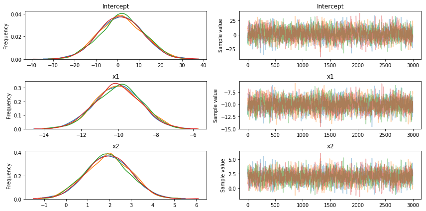
These are results obtained with the standard Pymc3 sampler (NUTS):

The results are approximately what we expected: the maximum a posteriori (MAP) estimation coincides with the ‘beta’ parameters we used for data generation. Let us try now a minor modification to introduce ADVI inference in this example:
# Code is the same as in previous code block, except for:
from pymc3.variational.callbacks import CheckParametersConvergence

with model:
    fit = pm.fit(100_000, method='advi', callbacks=[CheckParametersConvergence()])

draws = fit.sample(2_000) # This will automatically check parameters convergence
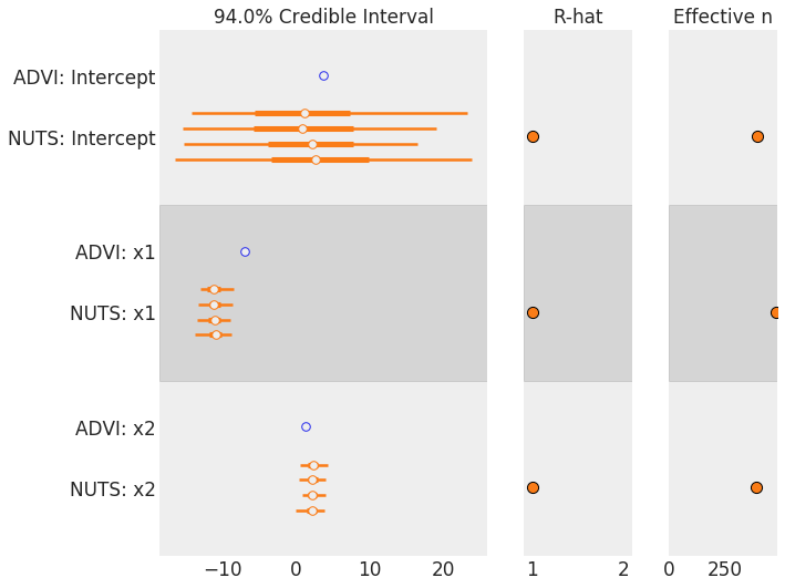
ADVI is considerably faster than NUTS, but what about accuracy? Instead of plotting bell curves again let us use this command to confront NUTS and ADVI results:
import arviz as az
az.plot_forest([draws, trace])

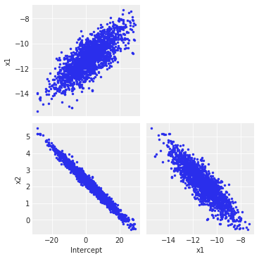
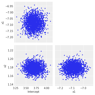
ADVI is clearly underestimating the variance, but it is fairly close to the mean of each parameter. Let us try to visualize the covariance structure of the model to understand where this lack of precision may come from (a big thank to colcarroll for pointing this out):
az.plot_pair(trace, figsize=(5, 5)) # Covariance plots for the NUTS trace

az.plot_pair(draws, figsize=(5, 5)) # Covariance plots for the NUTS trace

Clearly, ADVI does not capture (as expected) the interactions between variables because of the mean field approximation, and so it underestimates the overall variance by far (be advised: this is a particularly tricky example chosen to highlight this kind of behavior).
Conclusions
ADVI is a very convenient inferential procedure that let us characterize complex posterior distributions in a very short time (if compared to Gibbs/MCMC sampling). The solution it finds is a distribution which approximate the posterior, although it may not converge to the real posterior: for most cases this may not be a problem, but we may need to pay extra-attention in cases where the covariance structure of the variables is crucial (this example that uses Gaussian mixture models may clarify this concept)
References
- Black Box variational inference, Rajesh Ranganath, Sean Gerrish, David M. Blei, AISTATS 2014
- Keyonvafa’s blog
- Machine learning, a probabilistic perspective, by Kevin Murphy
- GLM in PyMC3
- ADVI publication on arXiv