Paper review & code: Deep Sets
Deep Sets, NIPS
This is a long overdue piece on a paper I read last year and found to be very interesting and easy to implement. It suggests a relatively simple way to structure deep nets in order to handle sets instead of ordered lists of elements. Despite this unimpressive description, it has important practical applications and its range of applicability goes far beyond what I thought of when I read the paper for the first time.
Sets in data are everywhere, and the class of models I will describe in the present post are in fact set to attain permutation invariance
of the inputs. An intuitive explanation of what a permutation invariant function is represented by the following chain of equalities
for a function f:
In the supervised setting modeling sets is relevant when dealing with mappings to a label that should be invariant to inputs ordering e.g. sets of objects in a scene, multi-agent reinforcement learning, estimation of population statistics…
In the unsupervised setting sets are relevant to tasks such as set/audience expansion, where given a set of objects that are similar to each other (e.g. set of words {lion, tiger, leopard}), our goal is to find new objects from a large pool of candidates such that the selected new objects are similar to the query (Zaheer et al., 2018).
Using the same notation of the DeepSets paper (Zaheer et al. 2018) a function operating on a input X is a valid set function
(i.e. invariant to the permutation of instances in X) iff it can be decomposed in the form
The two “sub”-functions and
are parameterized by neural networks,
so that shared branches of the net (defined by
)
process set elements independently, which are later pooled by
.
You can picture this process as well by regarding these two functions as
map ops followed by reduce.
The architecture
And this is a list of the required architectural elements we have just mentioned:
- Each input element of the set if transformed (possibily by several layers) of the ‘mapping’ function
- The resulting vectors are summed up (pooling operation) and the output is in turn transformed by the
network (which is the same as any other feed-forward neural network).
- An optional ‘branch’ of the neural network may be used to encode additional contextual information
related to the entire set. This effectively models the conditioning mapping
De Finetti’s theorem and the basis of exchangeability
The concept of permutation invariance is intimately connected with the concept of exchangeability in Bayesian statistics,
which is notably expressed in the De Finetti theorem.
This theorem states that exchangeable observations (i.e. members of a set) are conditionally independent relative to some
latent variable (). The formula is very clear in this regard:
In order to show how this formulation relates to the definition reported above of a permutation-invariant function, Zaheer et al. consider exponential families with conjugate priors (so that we can analytically calculate the integral). In this case the prior distribution is defined as:
and the likelihood as:
It is now possible to marginalize out the latent variable
and observe the resulting functional form, which looks exactly as the one listed above when defining the structure of our
permutation invariant neural network (just think of
and
):
The code
Let us now implement a simple experiment that is also reported in the original Deep Sets publication. A neural network receives in input a set of MNIST images (28 x 28 pixels) and needs to compute their numerical sum. In this experiment, the model is trained end-to-end in order to interpret the identity of the numbers in the input images and to produce their sum after aggregation (pooling). The number of images to be used (the input set) is itself a variable, in this simple example though it will be restricted to 3.
The structure of the neural net consists of an image-processing part which condense the information contained in the input image
(as usual through subsequent convolutional layers) and a feed-forward neural net after pooling (the sum operation) which transforms
the vector into the output number.
Let us start by sourcing the data from with tf APIs:
import tensorflow as tf
(x_train, y_train), (x_test, y_test) = tf.keras.datasets.mnist.load_data()
Next, we create a training/test set by sampling random triplets of numbers and computing their sum:
import numpy as np
from typing import List, Tuple
from tqdm import tqdm_notebook as tqdm

def extract_image_set(x_data: np.array, y_data :np.array, agg_fun=np.sum, n_images=3) -> Tuple[np.array, np.array]:
  """
  Extract a single set of images with corresponding target
  :param x_data
  """
  idxs = np.random.randint(low=0, high=len(x_data)-1, size=n_images)
  return x_data[idxs], agg_fun(y_data[idxs])


def generate_dataset(n_samples: int, x_data: np.array, y_data :np.array, agg_fun=np.sum, n_images=3) -> Tuple[List[List[np.array]], np.array]:
  """
  :return X,y in format suitable for training/prediction
  """
  generated_list = [extract_image_set(x_data, y_data, agg_fun, n_images) for i in tqdm(range(n_samples))]
  X, y = [i[0] for i in generated_list], np.array([t[1] for t in generated_list])
  output_lists = [[] for i in range(n_images)]
  for image_idx in range(n_images):
    for sample_idx in range(n_samples):
      output_lists[image_idx].append(np.expand_dims(X[sample_idx][image_idx], axis=2))
  return output_lists, y

X_train_data, y_train_data = generate_dataset(n_samples=100000, x_data=x_train, y_data=y_train, n_images=3)
X_test_data, y_test_data = generate_dataset(n_samples=20000, x_data=x_test, y_data=y_test, n_images=3)
And just to have an idea of what the dataset looks like we can create this visualization:
import matplotlib.pyplot as plt
%matplotlib inline

n_sample_viz, n_images = 3, 3

fig, axes = plt.subplots(nrows=n_sample_viz, ncols=n_images, figsize=(9.0, 9.0))

for sample_idx in range(n_sample_viz):
  for im_idx in range(n_images):
    axes[sample_idx, im_idx].imshow(X_train_data[im_idx][sample_idx][:, :, 0], cmap='Greys')
    axes[sample_idx, im_idx].axis('off')
    if im_idx==0:
      axes[sample_idx, 0].set_title('               Sum value for this row is {}'.format(y_train_data[sample_idx]),
                                    fontsize=15, loc='left')<img src="deepsets/numbers.png" alt="Image not found" width="500"/>
And now the network structure. In this simple example notice in particular the shared portion of the model (named feature_ext_model)
which processes in parallel the input images. The pooling operation in this model is the Add function that simply sums the values taken by
the output vectors.
from tensorflow.keras.layers import Dense
from tensorflow.keras.layers import Input
from tensorflow.keras.models import Model
from tensorflow.keras.layers import Conv2D
from tensorflow.keras.layers import MaxPooling2D
from tensorflow.keras.layers import Flatten
from tensorflow.keras.layers import Dropout
from tensorflow.keras.layers import Add
from tensorflow.keras.optimizers import Adam

import os, datetime

input_shape = (28, 28, 1)
filters = 64
kernel_size = 3

# Shared portion of the network
input_image = Input(shape=input_shape)

y = Conv2D(32, kernel_size=(3, 3),
           activation='relu',
           input_shape=input_shape)(input_image)
y = Conv2D(64, (3, 3), activation='relu')(y)
y = MaxPooling2D(pool_size=(2, 2))(y)
y = Dropout(0.25)(y)
y = Flatten()(y)
output_vec = Dense(128, activation='relu')(y)

feature_ext_model = Model(input_image, output_vec)

image_1, image_2, image_3 = Input(shape=input_shape), Input(shape=input_shape), \
                            Input(shape=input_shape)
outputs_1, outputs_2, outputs_3 = feature_ext_model(image_1), feature_ext_model(image_2), feature_ext_model(image_3)

y = Add()([outputs_1, outputs_2, outputs_3])
y = Dense(64, activation='relu')(y)
y = Dense(32, activation='relu')(y)
encoded = Dense(1)(y)

model = Model([image_1, image_2, image_3], encoded)
adam = Adam()
model.compile(optimizer=adam, loss='mae')

logdir = os.path.join("logs", datetime.datetime.now().strftime("%Y%m%d-%H%M%S"))
tensorboard_callback = tf.keras.callbacks.TensorBoard(logdir, histogram_freq=1)

model.fit(x=X_train_data, y=y_train_data,
          epochs=10, batch_size=64)
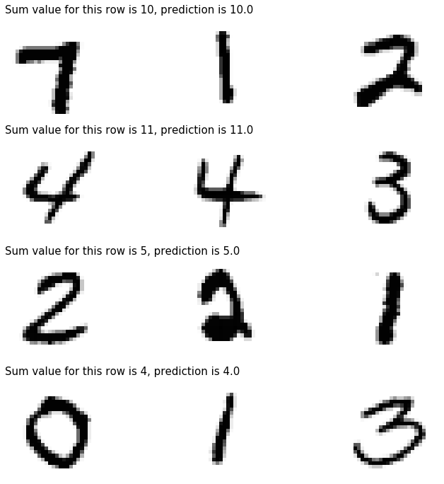
The trained model can now be used for prediction and we can visualize some random samples:
prediction = model.predict(x=X_test_data)

import matplotlib.pyplot as plt
%matplotlib inline

n_sample_viz, n_images = 4, 3

fig, axes = plt.subplots(nrows=n_sample_viz, ncols=n_images, figsize=(12.0, 12.0))
for sample_idx in range(n_sample_viz):
  for im_idx in range(n_images):
    axes[sample_idx, im_idx].imshow(X_test_data[im_idx][sample_idx][:, :, 0], cmap='Greys')
    axes[sample_idx, im_idx].axis('off')
    if im_idx==0:
      axes[sample_idx, 0].set_title('Sum value for this row is {}, prediction is {}'.format(y_test_data[sample_idx], round(prediction[sample_idx][0])),
                                    fontsize=15, loc='left')
Conclusion
The prediction accuracy on this simple dataset is of course very high, and it is safe to say that we do not need more complicated models to address problems like these.
Nonetheless, the simplistic pooling operation that we are using in this case (the sum) does not model interactions
between elements in the sets, giving way to (relevant) information loss. In the next post I will talk about (and provide a TF implementation of) the Set transformer,
which is an interesting work based on self-attention that models permutation-invariant function
while preserving higher-order interactions between members of input sets.
Reference
- https://www.inference.vc/deepsets-modeling-permutation-invariance/
- https://arxiv.org/pdf/1703.06114.pdf
Equation editor
- https://www.codecogs.com/latex/eqneditor.php (Latin Modern, 12pts, 150 dpi)